SAT Work Log 5

By Michal Jagodzinski - Work Log - April 17th, 2023

Hello and welcome back to Star Coffee! This is going to be another shorter post as I have been a bit busy lately. In this post, I go over some new updates on the orbital dynamics component of the Satellite Analysis Toolkit. Let's get into it.

Improving the Orbital Dynamics System

Firstly, I fixed a small "bug" or typing mistake regarding the OrbitalSystem struct I defined in SAT Work Log 3. There, I defined the struct as:

struct OrbitalSystem{T<:Number, Quant<:Number}
    type::String
    eqns::Vector{Equation}
    system::ODESystem
    problem::ODEProblem
    u₀::Dict{Num, Quant}
    params::Dict{Num, Quant}
    tspan::Vector{T}
end

I wrote this when I was still learning structs, so it wasn't defined in the clearest way. This time around I rewrote the Quant types as type unions instead:

struct OrbitalSystem{T<:Number}
    type::String
    orbital_bodies::Dict{String, OrbitalBody}
    eqns::Vector{Equation}
    system::ODESystem
    problem::ODEProblem
    u₀::Dict{Num, Union{T, Quantity{T}}}
    params::Dict{Num, Union{T, Quantity{T}}}
    tspan::Vector{T}
end

This version is written a little clearer I think. For context, I want users to be able to define orbital systems with or without Unitful.jl units, hence the type union. You may notice the addition of the orbital_bodies field. I am implementing a new struct called OrbitalBody, which contains all the information about a specific body in an orbital system. It is defined as:

mutable struct BodyState{T<:Number}
    x::Union{T, Quantity{T}}
    y::Union{T, Quantity{T}}
    z::Union{T, Quantity{T}}
    ẋ::Union{T, Quantity{T}}
    ẏ::Union{T, Quantity{T}}
    ż::Union{T, Quantity{T}}
end

mutable struct OrbitalBody{T<:Number}
    name::String
    mass::Union{T, Quantity{T}}
    state::BodyState{T}
end

I created these structs to better organize information about orbital systems and to provide an interface for future interactive orbital dynamics tools. With the new OrbitalSystem definition, the constructor for a two-body system is:

function TwoBodySystem(
    u₀::Dict{Num, Quantity{T}},
    params::Dict{Num, Quantity{T}},
    tspan::Vector{T}
) where {T<:Number}

    @assert valtype(u₀) == valtype(params) "Numeric values in u₀ and params must be the same type"

    two_body_equations = LoadTwoBodyEquations()

    diffeq_two_body_system = structural_simplify(
        ODESystem(two_body_equations, t, name=:two_body_system)
    )

    prob = ODEProblem(
        diffeq_two_body_system,
        remove_units(u₀),
        tspan,
        remove_units(params),
        jac=true
    )

    orbital_bodies = Dict(
        "Body 1" => OrbitalBody(
            "Body 1",
            params[m₁],
            BodyState(
                u₀[x₁],
                u₀[y₁],
                u₀[z₁],
                u₀[ẋ₁],
                u₀[ẏ₁],
                u₀[ż₁],
            )
        ),
        "Body 2" => OrbitalBody(
            "Body 2",
            params[m₂],
            BodyState(
                u₀[x₂],
                u₀[y₂],
                u₀[z₂],
                u₀[ẋ₂],
                u₀[ẏ₂],
                u₀[ż₂],
            )
        ),
    )

    return OrbitalSystem{T}(
        "Two-Body System",
        orbital_bodies,
        two_body_equations,
        diffeq_two_body_system,
        prob,
        u₀,
        params,
        tspan
    )
end

I also implemented constructors for the OrbitalSystem based on the number of inputted OrbitalBody structs, e.g., for a two-body system:

function OrbitalSystem(
    body_1::OrbitalBody{T},
    body_2::OrbitalBody{T},
    tspan::Vector{T};
    G_val=6.6743e-11
) where {T<:Number}

    orbital_bodies = Dict(
        body_1.name => body_1,
        body_2.name => body_2
    )

    two_body_equations = LoadTwoBodyEquations()

    diffeq_two_body_system = structural_simplify(
        ODESystem(two_body_equations, t, name=:two_body_system)
    )

    u₀ = Dict(
        x₁ => body_1.state.x,
        y₁ => body_1.state.y,
        z₁ => body_1.state.z,
        ẋ₁ => body_1.state.ẋ,
        ẏ₁ => body_1.state.ẏ,
        ż₁ => body_1.state.ż,
        x₂ => body_2.state.x,
        y₂ => body_2.state.y,
        z₂ => body_2.state.z,
        ẋ₂ => body_2.state.ẋ,
        ẏ₂ => body_2.state.ẏ,
        ż₂ => body_2.state.ż
    )

    params = Dict(
        G => G_val,
        m₁ => body_1.mass,
        m₂ => body_2.mass
    )

    if (typeof(body_1.mass) == typeof(body_2.mass)) && typeof(body_1.mass) <: Quantity{T}
        if !(typeof(G_val) <: Quantity{T})
            params[G] = G_val * 1u"N*m^2/kg^2"
        end

        prob = ODEProblem(
            diffeq_two_body_system,
            remove_units(u₀),
            tspan,
            remove_units(params),
            jac=true
        )
    else
        prob = ODEProblem(
            diffeq_two_body_system,
            u₀,
            tspan,
            params,
            jac=true
        )
    end

    return OrbitalSystem{T}(
        "Two-Body System",
        orbital_bodies,
        two_body_equations,
        diffeq_two_body_system,
        prob,
        u₀,
        params,
        tspan
    )
end

Simulations with Improved Orbital Dynamics System

Now a simple plotting example using this new system:

using GLMakie, ModelingToolkit, DifferentialEquations, Unitful
GLMakie.activate!()

include("TwoBody.jl")

body1 = OrbitalBody(
    "Test 1",
    10e26u"kg",
    BodyState(0.0u"m", 0.0u"m", 0.0u"m", 10.0u"km/s", 20.0u"km/s", 30.0u"km/s")
)

body2 = OrbitalBody(
    "Test 2",
    10e26u"kg",
    BodyState(3000.0u"km", 0.0u"m", 0.0u"m", 0.0u"m/s", 40.0u"km/s", 0.0u"m/s")
)

t, x₁, y₁, z₁, ẋ₁, ẏ₁, ż₁, x₂, y₂, z₂, ẋ₂, ẏ₂, ż₂, r, D, G, m₁, m₂ = LoadTwoBodyVariables()

two_body_system = OrbitalSystem(body1, body2, [0.0, 480.0])
two_body_sol = SolveOrbitalSystem(two_body_system, Tsit5())

fig = Figure(resolution=(1500,1500)); display(fig);
ax1 = Axis3(fig[1,1])

times = 0.0:0.1:480.0
lines!(ax1, interp_sol(two_body_sol, [x₁, y₁, z₁], times)..., label="Mass 1")
lines!(ax1, interp_sol(two_body_sol, [x₂, y₂, z₂], times)..., label="Mass 2")
axislegend(ax1)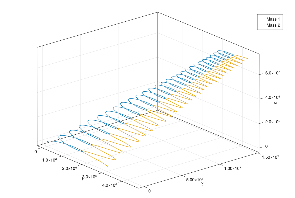

Alternatively, using the previous system:

using GLMakie, ModelingToolkit, DifferentialEquations, Unitful
GLMakie.activate!()

include("TwoBody.jl")

t, x₁, y₁, z₁, ẋ₁, ẏ₁, ż₁, x₂, y₂, z₂, ẋ₂, ẏ₂, ż₂, r, D, G, m₁, m₂ = LoadTwoBodyVariables()

two_body_example_u₀ = Dict(
    x₁ => 0.0u"m",
    y₁ => 0.0u"m",
    z₁ => 0.0u"m",
    ẋ₁ => 10.0u"km/s",
    ẏ₁ => 20.0u"km/s",
    ż₁ => 30.0u"km/s",
    x₂ => 3000.0u"km",
    y₂ => 0.0u"m",
    z₂ => 0.0u"m",
    ẋ₂ => 0.0u"m/s",
    ẏ₂ => 40.0u"km/s",
    ż₂ => 0.0u"m/s"
)

two_body_example_p = Dict(
    G => 6.6743e-11u"N*m^2/kg^2",
    m₁ => 10e26u"kg",
    m₂ => 10e26u"kg"
)

two_body_system = TwoBodySystem(two_body_example_u₀, two_body_example_p, [0.0, 480.0])
two_body_sol = SolveOrbitalSystem(two_body_system, Tsit5())

fig = Figure(resolution=(1500,1500)); display(fig);
ax1 = Axis3(fig[1,1])

times = 0.0:0.1:480.0
lines!(ax1, interp_sol(two_body_sol, [x₁, y₁, z₁], times)..., label="Mass 1")
lines!(ax1, interp_sol(two_body_sol, [x₂, y₂, z₂], times)..., label="Mass 2")
axislegend(ax1)

Both methods result in the exact same OrbitalSystem. I think having a choice of methods is a good idea. Using the OrbitalBody method is better for integrating with interactive tools, whereas using the TwoBodySystem constructor is better for users directly running simulations manually.

I needed to include the call to the LoadTwoBodyVariables() as the Symbolics.jl variables could be defined with or without units, and I don't want to assume units for every case. These variables have to be defined as the OrbitalSystem uses ODEs defined by these variables (see SAT Work Log 2 - Orbital Dynamics Work). To work with unitless values, LoadTwoBodyVariablesUnitless() is called instead.

I realize having to define the system variables in the main scope in this way is quite clunky. Unfortunately this is the best way I found to do this at the moment. I am thinking of defining macros to do this automatically, but I don't know enough about macros to implement this just yet.

I also wrote a simple helper function to automatically apply and return the interpolated values of inputted variables to an ODE solution, which I use above:

function interp_sol(
    solution::ODESolution,
    vars::Vector{Num},
    times::Union{StepRangeLen, Vector}
)

    sol_interp = solution(times)
    return [sol_interp[var] for var in vars]
end

Wrapping Up

Thanks for reading this short post! I hope to have more exciting work to showcase soon. I want a good foundation defined before building more complex tools, so I believe this type of work is necessary. Until next time.