SAT Work Log 3

By Michal Jagodzinski - Work Log - April 7th, 2023

Welcome back to Star Coffee! In this Satellite Analysis Toolkit work log I discuss the future design of the SAT system and implement some more orbital dynamics. Let's get into it.

Pondering SAT System Design

I am thinking of implementing a universal Satellite object with functionality throughout SAT. For example, you can design a mission for a Satellite in MissionPlanner, analyze the ground tracks of its orbits in GroundTracker, etc. This would also allow for saving and sharing analyses.

I will probably also define a Mission struct in order to define the state of a Satellite at a given stage in its lifetime. Each Satellite would have one or more Mission structs to define the entire long-term mission of that specific satellite.

In general I want to make use of structs to try and create more of a 'coherent' system. When working with SAT, I don't want to have to memorize the inner workings of the code. I want to develop a nice, high-level interface to work with.

More Orbital Dynamics

The Three-Body Problem

This scenario is the same as the two-body problem except with the introduction of another body that gravitationally influences the two others, and is in turn influenced by the others. The differential equations for the three-body problem are defined as:

$$\ddot{\mathbf{r}}_{1} = \begin{bmatrix} \ddot{x}_{1} \\ \ddot{y}_{1} \\ \ddot{z}_{1} \end{bmatrix} = \begin{bmatrix} \dfrac{G m_{2} (x_{2} - x_{1})}{r_{12}^3} + \dfrac{G m_{3} (x_{3} - x_{1})}{r_{13}^3} \\ \dfrac{G m_{2} (y_{2} - y_{1})}{r_{12}^3} + \dfrac{G m_{3} (y_{3} - y_{1})}{r_{13}^3} \\ \dfrac{G m_{2} (z_{2} - z_{1})}{r_{12}^3} + \dfrac{G m_{3} (z_{3} - z_{1})}{r_{13}^3} \end{bmatrix}$$ $$\ddot{\mathbf{r}}_{2} = \begin{bmatrix} \ddot{x}_{2} \\ \ddot{y}_{2} \\ \ddot{z}_{2} \end{bmatrix} = \begin{bmatrix} \dfrac{G m_{1} (x_{1} - x_{2})}{r_{12}^3} + \dfrac{G m_{3} (x_{3} - x_{2})}{r_{3}^3} \\ \dfrac{G m_{1} (y_{1} - y_{2})}{r_{12}^3} + \dfrac{G m_{3} (y_{3} - y_{2})}{r_{23}^3} \\ \dfrac{G m_{1} (z_{1} - z_{2})}{r_{12}^3} + \dfrac{G m_{3} (z_{3} - z_{2})}{r_{23}^3} \end{bmatrix}$$ $$\ddot{\mathbf{r}}_{3} = \begin{bmatrix} \ddot{x}_{3} \\ \ddot{y}_{3} \\ \ddot{z}_{3} \end{bmatrix} = \begin{bmatrix} \dfrac{G m_{1} (x_{1} - x_{3})}{r_{13}^3} + \dfrac{G m_{2} (x_{2} - x_{3})}{r_{23}^3} \\ \dfrac{G m_{1} (y_{1} - y_{3})}{r_{13}^3} + \dfrac{G m_{2} (y_{2} - y_{3})}{r_{23}^3} \\ \dfrac{G m_{1} (z_{1} - z_{3})}{r_{13}^3} + \dfrac{G m_{2} (z_{2} - z_{3})}{r_{23}^3} \end{bmatrix}$$

Where

$$\begin{align*} r_{12} &= \sqrt{ (x_{2} - x_{1})^2 + (y_{2} - y_{1})^2 + (z_{2} - z_{1})^2 } \\ r_{13} &= \sqrt{ (x_{3} - x_{1})^2 + (y_{3}-y_{1})^2 + (z_{3}-z_{1})^2 } \\ r_{23} &= \sqrt{ (x_{3} - x_{2})^2 + (y_{3}-y_{2})^2 + (z_{3}-z_{2})^2 } \end{align*}$$

The implementation of this system in Julia is similar to the two-body problem, so see my previous post if you want some more details. Starting off with the required libraries and a helper function:

using Plots, ModelingToolkit, DifferentialEquations, Unitful

function remove_units(p::Dict)
    Dict(k => Unitful.ustrip(ModelingToolkit.get_unit(k), v) for (k, v) in p)
end

Next, the variables and parameters of the system:

@variables(begin
    t, [unit=u"s"],
    x₁(t), [unit=u"m"],
    y₁(t), [unit=u"m"],
    z₁(t), [unit=u"m"],
    ẋ₁(t), [unit=u"m/s"],
    ẏ₁(t), [unit=u"m/s"],
    ż₁(t), [unit=u"m/s"],
    x₂(t), [unit=u"m"],
    y₂(t), [unit=u"m"],
    z₂(t), [unit=u"m"],
    ẋ₂(t), [unit=u"m/s"],
    ẏ₂(t), [unit=u"m/s"],
    ż₂(t), [unit=u"m/s"],
    x₃(t), [unit=u"m"],
    y₃(t), [unit=u"m"],
    z₃(t), [unit=u"m"],
    ẋ₃(t), [unit=u"m/s"],
    ẏ₃(t), [unit=u"m/s"],
    ż₃(t), [unit=u"m/s"],
    r₁₂(t), [unit=u"m"],
    r₁₃(t), [unit=u"m"],
    r₂₃(t), [unit=u"m"]
end)

D = Differential(t)

@parameters G [unit=u"N*m^2/kg^2"] m₁ [unit=u"kg"] m₂ [unit=u"kg"] m₃ [unit=u"kg"]

Next, the equations of the system:

three_body_equations = [
    r₁₂ ~ sqrt((x₂ - x₁)^2 + (y₂ - y₁)^2 + (z₂ - z₁)^2),
    r₁₃ ~ sqrt((x₃ - x₁)^2 + (y₃ - y₁)^2 + (z₃ - z₁)^2),
    r₂₃ ~ sqrt((x₃ - x₂)^2 + (y₃ - y₂)^2 + (z₃ - z₂)^2),

    D(x₁) ~ ẋ₁,
    D(y₁) ~ ẏ₁,
    D(z₁) ~ ż₁,
    D(ẋ₁) ~ G*m₂*(x₂ - x₁)/r₁₂^3 + G*m₃*(x₃ - x₁)/r₁₃^3,
    D(ẏ₁) ~ G*m₂*(y₂ - y₁)/r₁₂^3 + G*m₃*(y₃ - y₁)/r₁₃^3,
    D(ż₁) ~ G*m₂*(z₂ - z₁)/r₁₂^3 + G*m₃*(z₃ - z₁)/r₁₃^3,

    D(x₂) ~ ẋ₂,
    D(y₂) ~ ẏ₂,
    D(z₂) ~ ż₂,
    D(ẋ₂) ~ G*m₁*(x₁ - x₂)/r₁₂^3 + G*m₃*(x₃ - x₂)/r₂₃^3,
    D(ẏ₂) ~ G*m₁*(y₁ - y₂)/r₁₂^3 + G*m₃*(y₃ - y₂)/r₂₃^3,
    D(ż₂) ~ G*m₁*(z₁ - z₂)/r₁₂^3 + G*m₃*(z₃ - z₂)/r₂₃^3,

    D(x₃) ~ ẋ₃,
    D(y₃) ~ ẏ₃,
    D(z₃) ~ ż₃,
    D(ẋ₃) ~ G*m₁*(x₁ - x₃)/r₁₃^3 + G*m₂*(x₂ - x₃)/r₂₃^3,
    D(ẏ₃) ~ G*m₁*(y₁ - y₃)/r₁₃^3 + G*m₂*(y₂ - y₃)/r₂₃^3,
    D(ż₃) ~ G*m₁*(z₁ - z₃)/r₁₃^3 + G*m₂*(z₂ - z₃)/r₂₃^3,
]

diffeq_three_body_system = ODESystem(
    three_body_equations,
    t,
    name=:three_body_system
) |> structural_simplify

Example initial conditions:

u₀ = Dict(
    x₁ => -0.97138u"m",
    y₁ => 0.0u"m",
    z₁ => 0.0u"m",
    ẋ₁ => 0.0u"m/s",
    ẏ₁ => -1.37584u"m/s",
    ż₁ => 0.0u"m/s",
    x₂ => 1.0u"m",
    y₂ => 0.0u"m",
    z₂ => 0.0u"m",
    ẋ₂ => 0.0u"m/s",
    ẏ₂ => -0.34528u"m/s",
    ż₂ => 0.0u"m/s",
    x₃ => 0.0u"m",
    y₃ => 0.0u"m",
    z₃ => 0.0u"m",
    ẋ₃ => 0.0u"m/s",
    ẏ₃ => 1.519362144u"m/s",
    ż₃ => 0.0u"m/s",
)

p = Dict(
    G => 1.0u"N*m^2/kg^2",
    m₁ => 0.5312u"kg",
    m₂ => 2.2837u"kg",
    m₃ => 1u"kg"
)

Finally, defining the problem and solving:

three_body_problem = ODEProblem(
    diffeq_three_body_system,
    remove_units(u₀),
    [0.0, 10.0],
    remove_units(p),
    jac=true
)

three_body_sol = solve(three_body_problem, Vern7())

Plotting the results:

interp = three_body_sol(0.0:0.001:10.0)

plot(interp[x₁], interp[y₁], interp[z₁], size=(600,500), dpi=300)
plot!(interp[x₂], interp[y₂], interp[z₂])
plot!(interp[x₃], interp[y₃], interp[z₃])

Circular Restricted Three-Body Problem

Next, a special case of the three-body problem. The circular restricted three-body system is the case when two bodies $m_1$ and $m_2$ orbiting each-other at a constant distance $r_{12}$, with a significantly smaller mass moving throughout this system. A real-life example of this is the Earth-Moon system with a satellite moving throughout it. This case of the three-body problem is useful when analyzing missions that transfer between the Earth and the Moon.

The differential equations describing the movement of the smaller mass/satellite are:

$$\begin{align*} \ddot{x} &= 2 \Omega \dot{y} + \Omega^2 x - \frac{\mu_{1}}{r_{1}^3}(x + \pi_{2} r_{12}) - \frac{\mu_{2}}{r_{2}^3}(x - \pi_{1}r_{12}) \\ \ddot{y} &= \Omega^2 y - 2 \Omega \dot{x} - \frac{\mu_{1}}{r_{1}^3}y - \frac{\mu_{2}}{r_{2}^3}y \\ \ddot{z} &= -\frac{\mu_{1}}{r_{1}^3}z - \frac{\mu_{2}}{r_{2}^3}z \end{align*}$$

Where

$$\begin{align*} \Omega &= \sqrt{ \dfrac{G(m_{1} + m_{2})}{r_{12}^3} } \\ \mu_{1} &= G m_{1} \\ \mu_{2} &= G m2 \\ \pi_{1} &= \frac{m_{1}}{m_{1}+m_{2}} \\ \pi_{2} &= \frac{m_{2}}{m_{1}+m_{2}} \\ r_{1} &= \sqrt{ (x + \pi_{2}r_{12})^2 + y^2 + z^2 } \\ r_{2} &= \sqrt{ (x - \pi_{1}r_{12})^2 + y^2 + z^2 } \end{align*}$$

For the CR3BP, I will be implementing the Earth-Moon system, however the system can be parameterized to model any arbitrary system. First, defining some constants:

const mₑ = 5.97e24
const mₘ = 7.3459e22
const G_val = 6.6743e-11

const r₁₂_val = 384400e3

const Ω = sqrt(G_val * (mₑ + mₘ)/r₁₂_val^3)
const μ₁ = G_val*mₑ
const μ₂ = G_val*mₘ

const π₁ = mₑ/(mₑ + mₘ)
const π₂ = mₘ/(mₑ + mₘ)

Next, the system variables (note I am introducing the ti and Di variables to prevent compatibility errors between the circular restricted and general three-body propagators):

@variables(begin
    ti,
    x(ti),
    y(ti),
    z(ti),
    ẋ(ti),
    ẏ(ti),
    ż(ti),
    r₁(ti),
    r₂(ti)
end)

Di = Differential(ti)

The system equations:

earth_moon_cr_three_body_equations = [
    r₁ ~ sqrt((x + π₂*r₁₂_val)^2 + y^2 + z^2),
    r₂ ~ sqrt((x - π₁*r₁₂_val)^2 + y^2 + z^2),

    Di(x) ~ ẋ,
    Di(y) ~ ẏ,
    Di(z) ~ ż,

    Di(ẋ) ~ 2*Ω*ẏ + x*Ω^2 - (x + π₂*r₁₂_val)*μ₁/r₁^3 - (x - π₁*r₁₂_val)*μ₂/r₂^3,
    Di(ẏ) ~ y*Ω^2 - 2*Ω*ẋ - y*μ₁/r₁^3 - y*μ₂/r₂^3,
    Di(ż) ~ -z*μ₁/r₁^3 - z*μ₂/r₂^3,
]

earth_moon_cr_three_body_system = ODESystem(
    earth_moon_cr_three_body_equations,
    ti,
    name=:earth_moon_cr_three_body_system
) |> structural_simplify

Defining the conditions for a lunar fly-by:

u₀ = Dict(
    x => -4671e3,
    y => -6378e3 - 200e3,
    z => 0.0,
    ẋ => 10.9148e3 * cos(deg2rad(19)),
    ẏ => -10.9148e3 * sin(deg2rad(19)),
    ż => 0.0
)

Finally once more, defining the problem and solving:

earth_moon_cr_three_body_problem = ODEProblem(
    earth_moon_cr_three_body_system,
    u₀,
    [0.0, 3.4 * 24 * 60 * 60],
    [],
    jac=true
)

cr_three_body_sol = solve(earth_moon_cr_three_body_problem, Tsit5())

Now we can plot the result:

function circle(x, y, r)
    θ = LinRange(0, 2*π, 500)
    x .+ r*sin.(θ), y .+ r*cos.(θ)
end

cr3bp_interp = cr_three_body_sol(0.0 : 50 : 3.4 * 24 * 60 * 60)

plot(
    cr3bp_interp[x] ./ 1e3, cr3bp_interp[y] ./ 1e3,
    xlabel="x (km)", ylabel="y (km)",
    size=(800,500),
    aspect_ratio=:equal,
    label=""
)

plot!(
    circle(-4671, 0, 6378),
    seriestype = [:shape,],
    lw=0.5, c = :lightblue, fillalpha=0.5,
    label=""
)

plot!(
    circle(-4671 + 384400, 0, 1737.4),
    seriestype = [:shape,],
    lw=0.5, c = :gray, fillalpha=0.5,
    label=""
)

Pretty sick.

You may have noticed that I did not include units with the definition of this orbit type. As with the previous types, I've tried implementing Unitful.jl units into the system definition. However, this orbit type just does not play nicely with units. The first issue I encountered was:

MethodError: *(::Unitful.Quantity{Float64, 𝐓⁻¹, Unitful.FreeUnits{(rad, s⁻¹), 𝐓⁻¹, nothing}}, ::Symbolics.Num) is ambiguous.

I've tried fixing this issue and another issue with division as well by reading through a GitHub issue thread, which suggested to overload the multiplication operator:

import Base:*
*(x::Unitful.AbstractQuantity,y::Num) =  Quantity(x.val*y, unit(x))
*(y::Num,x::Unitful.AbstractQuantity) = x*y

import Base:/
/(x::Unitful.AbstractQuantity,y::Num) =  Quantity(x.val/y, unit(x))
/(y::Num,x::Unitful.AbstractQuantity) = y/x

This fixed the initial error, but then I was getting a DimensionError related to the $\Omega$ variable:

DimensionError: 5.33076e-6ẏ(t) rad s⁻¹ and 7.104250544399999e-12x(t) rad² s⁻² are not dimensionally compatible.

Getting rid of the units from $\Omega$ causes yet another error:

TypeError: non-boolean (Symbolics.Num) used in boolean context

At this point I just decided to wait until Unitful.jl and ModelingToolkit.jl had time to update and hopefully work together better. Until then, the CR3BP propagator will not include units.

Integrating the Orbital Systems with SAT

With the major orbit dynamics systems defined, my next goal is to integrate them properly into SAT. I want to create a general interface to work with the three systems and potential future ones. Here is my initial attempt at a universal orbital system format to encode the information about a specific system, as well as some constructors for a two-body system:

struct OrbitalSystem{T<:Number, Quant<:Number}
    type::String
    eqns::Vector{Equation}
    system::ODESystem
    problem::ODEProblem
    u₀::Dict{Num, Quant}
    params::Dict{Num, Quant}
    tspan::Vector{T}
end

function Base.show(io::IO, system::OrbitalSystem)
    out_string = """Orbital System Model: $(system.type)

    Initial Conditions:
    $(system.u₀)

    Parameters:
    $(system.params)
    """

    println(out_string)
end

function TwoBodySystem(
    u₀::Dict{Num, Quantity{T}},
    params::Dict{Num, Quantity{T}},
    tspan::Vector{T}
) where {T<:Number}
    @assert valtype(u₀) == valtype(params) "Numeric values in u₀ and params must be the same type"

    prob = ODEProblem(
        diffeq_two_body_system,
        remove_units(u₀),
        tspan,
        remove_units(params),
        jac=true
    )

    return OrbitalSystem{T, Quantity{T}}(
        "Two-Body System",
        two_body_equations,
        diffeq_two_body_system,
        prob,
        u₀,
        params,
        tspan
    )
end

function TwoBodySystem(
    u₀::Dict{Num, T},
    params::Dict{Num, T},
    tspan::Vector{T}
) where {T<:Number}
    @assert valtype(u₀) == valtype(params) "Numeric values in u₀ and params must be the same type"

    @warn "Warning: It is recommended to use Unitful.jl units when working with SAT"

    prob = ODEProblem(
        diffeq_two_body_system,
        u₀,
        tspan,
        params,
        jac=true
    )

    return OrbitalSystem{T, T}(
        "Two-Body System",
        two_body_equations,
        diffeq_two_body_system,
        prob,
        u₀,
        params,
        tspan
    )
end

function SolveOrbitalSystem(system::OrbitalSystem, solver::Union{DEAlgorithm,Nothing}; solver_args...)
    return solve(system.problem, solver; solver_args...)
end

As can be seen, I am making sure that the initial values and parameter variables are a consistent datatype, the same as I have been using during development of the orbital systems. I want to enforce the use of units as well, for applying conversions and other functionality. In addition, I am using multiple dispatch to include an option to define a system without units, though this prints a warning advising against this. This struct also provides potential users access to the equations, the ODESystem, and ODEProblem variables if they want to use those specifically.

I also want to implement a way to ensure that the u₀ and params variables provided to the constructors are properly set, i.e.,

• u₀ contains all the required variables (x₁, ẋ₁, etc.) and params contains all the required parameters (G, m₁, etc.)

• If using units, also ensuring that the units are correct, i.e. G is in $\text{N} \; \text{m}^2 / \text{kg}^2$, ẋ₁ is in $\text{m}/\text{s}$, etc.

I think this emphasis on validation ensures that no silly mistakes are made, and the user is being careful with their inputs. It also provides reassurance that the calculations done by SAT themselves are valid.

The SolveOrbitalSystem function is probably not necessary, but it just simplifies the call to the solve function by removing the need for the user to specify the problem of the system themselves.

Testing Orbital Dynamics Integration

With the OrbitalSystem struct, it is now pretty convenient to define and solve the two-body problem. For a simple plotting example using Makie.jl:

two_body_system = TwoBodySystem(
    two_body_example_u₀,
    two_body_example_p,
    two_body_example_tspan
)

two_body_sol = SolveOrbitalSystem(two_body_system, Tsit5())

fig = Figure(resolution=(1500,1500))
ax1 = Axis3(fig[1,1])

lines!(
    ax1,
    sol_interp[x₁], sol_interp[y₁], sol_interp[z₁],
    label="Mass 1"
)

lines!(
    ax1,
    sol_interp[x₂], sol_interp[y₂], sol_interp[z₂],
    label="Mass 2"
)

axislegend(ax1)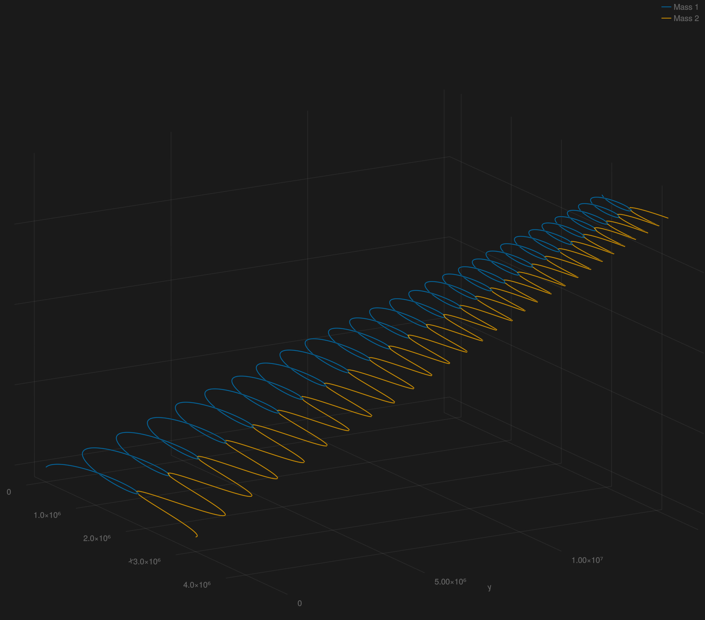

I will also write some more functions to further simplify workflows. For example, a function that automatically returns the vectors of interpolated values from the solution variable given the desired variables and a range of times.

Wrapping Up

Thanks for reading! It was fun adding more functionality to SAT. With the main orbital dynamics propagators defined I will focus more on building interactive tools that use them, as well as further refining the workflow of using the OrbitalSystem objects.

Thanks for reading! Until next time.